Volatility is lying: Why the vix underprices real risk?
Source: Nick Chong, Unsplash
Author: Mihail Gaydarov, Chief Financial Analyst
Volatility as a market indicator
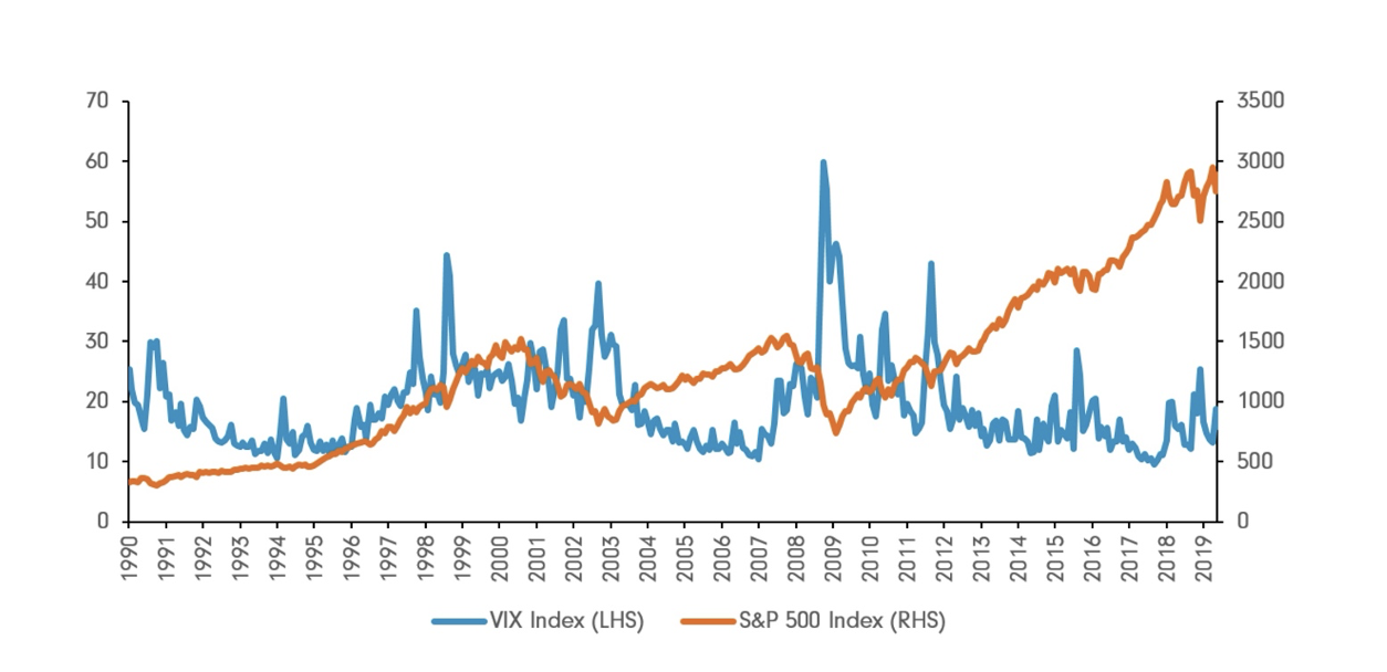
Periods of low market volatility are widely interpreted as signals of stability and safety. Through the course of history, such conditions have rarely been a reliable signal of safety. Researchers have found that on the contrary, prolonged periods often coincide with the steady accumulation of risk (Chen, Verousis, 2023) – through leverage, crowded positioning, and reduced sensitivity to price signals. A frequently mentioned illustration of this effect is a period known as the “Great Moderation”, during which macroeconomic factors and market volatility remained calm for years to come, while at the same time leverage, maturity mismatch and systematic fragility accumulated beneath the surface level security, ultimately contributing a fair share to the 2008 financial crisis.
More often than not, volatility is seen as an indicator to an investor whether the market is at risk or not. Where in fact we could argue that volatility as a tool is more of a reaction of the stock market rather than an indicator of hazard and safety.
In essence, a low volatility environment creates a poor sense of security among investors. This face-value stability gives ground to leverage encouragement, and investors are more prone to taking risk. Another point to be made here is that risk is accumulated structurally and not visibly through the index itself. More important risks like rising leverage, crowded positioning and liquidity mismatches are not presented at all (IMF, 2025). And ultimately, some investors use volatility as a diagnostic tool it was never designed to be.
This raises a critical question: if volatility does not measure risk, what does it actually measure?
What is market volatility at its core?
The primary distinction with arguably most consequence we can make here is that market volatility and investment risk are two very separate ideas. Firstly, volatility is a tool that measures price movement more than anything – how much has this stock change its price over a short/long period of time? We can consider volatility in the following matter – it is observable ex post and implied ex ante.
Source: Fidelity, Singapore
Whereas market risk concerns itself with the probability and magnitude of permanent loss on an investment position. Essentially, what happens if certain adverse scenarios materialise? Examples of such adverse scenarios we can consider wars, geopolitical conflicts and as of recent times trade wars.
If we need to word these points in a more simple, conceptual matter – a market can be volatile and at the same time solvent, and on the other hand calm yet very fragile (Knight, 1921).
Furthermore, we could argue that market volatility is symmetric, and on the contrary risk is asymmetric – meaning that a fluctuation of a stock “+10% and -10%” are treated as equivalents. A large upside might be seen as a threat where in fact it is completely opposite in some situations. For instance, if an investor plans to make a long-term position, temporal upside volatility does not constitute to losses, until the investment assets are capitalized. More often than not, when we look at compounding growth portfolios – high risk volatility portfolios are more prone to higher short-term gains, while the long-run steady volatility portfolios outpace high ones.
We must consider that a speculative bubble in a market with smooth upwards price trends could indicate low volatility and at the same time surge, a few months down the line. A distressed asset could be recovering and at the same time show very high volatility. If we observe energy stocks that experience steep declines in bear markets often rebound strongly, with some sectors showing a "V-shape" recovery in early 2023 after a 2022 decline, affirming the aforementioned claim.
What does VIX actually measure?
We discussed all the implications of The Volatility Index and how some investors might misinterpret the presented information, now we can confer on how the index itself is composed. Originally coined by The Chicago Board Option Exchange (CBOE) in 1993, the VIX utilizes a supply and demand principle to measure the traffic of S&P500 option purchases. In broader terms, we consider that when a player on the stock market feels a concern regarding the market itself, they engage in buying options for the stock position they hold, which in our case are the S&P 500 options. These options are used to hedge stock positions, limiting the maximum loss an investor can incur. By measuring the number of options bought, the index shows a direct relation. When investors feel insecure about the market, they purchase S&P 500 options, option demand rises, implied volatility rises – thus VIX experience an incline.
On the topic as why that happens, we must understand better as to what options are? Options are insurance / security positions on the targeted stock. In more technical terms they are financial derivative contracts that grant the right – but not the obligation to buy or sell an underlying asset at a predetermined price.
- Buying an option (call) – the holder makes money if the price goes up
- Selling an option (put) – the holder makes money if the price goes down
So, options exist to protect our investments by limiting the maximum loss to the premium of the option bought.
Why is volatility systematically suppressed?
It is important to note that Volatility is not just observed, but it is produced by market mechanics. In the modern times we live in a few mechanisms frame short term price fluctuations and more specifically delay the expression of risk.
Passive and Price-insensitive flows
As the growth of passive investment vehicles like ETFs and index funds continues, short term price dynamics are altered materially. Index funds and exchange traded products allocate capital mechanically, responding to inflows and outflows rather than to valuation or more specific firm information. While such mechanisms reduce transaction costs for a consumer, we have to keep in mind that they also reduce day-to-day price discovery for stock market shareholders.
Volatility is suppressed due to the continuous inflows of capital in shared securities that significantly smoothen price responsiveness. As a result of that, individual securities become much less responsive to information. Subsequently, this unresponsiveness creates a gap between the establishment of a stock market issue and the reaction of the individual asset itself, leading to the false sense of security among investors we have been discussing. And whenever the flows reverse the adjustment is very sudden and prices absorb the accumulated imbalances.
Volatility selling as a yield strategy
Volatility selling is especially seen as a substitute for carry strategies. Large institutions that control large scale assets use option selling in order to collect premium (profits) on them – creating an incentive for high volatility and fear. These large-scale enterprises utilize options as carry assets (income creating assets). The widespread adoption of this approach increases the supply of options and compresses implied volatility, reinforcing the perception of stability. However, volatility selling embeds convex exposure: gains accrue gradually during calm periods, while losses accelerate rapidly when volatility rises. In practice we observed this dynamic during the spike in Volatility in February 2018. Years of suppressed volatility and widespread short-volatility positioning unraveled abruptly, forcing rapid deleveraging and causing volatility to reprice violently over a matter of days. In essence, this approach is fruitful to such institutions because most days are calm and uneventful.
Above all, we can observe volatility as a mean reverting when it comes to this strategy. Mean reverting is a financial theory that operates on the suggestion that asset prices, returns, and volatility tend to return to their long-term average or historical mean over time. Put simply, extreme highs and lows are seen as temporary events. Even if there is a case of a “black swan” event on the stock market, these institutions rely on long-term average profits to stay in business.
Dealer hedging and stabilizing loops
Dealers are basically entities that trade options. Dealers that sell options are not directional investors. They are market participants that use strategies designed to generate absolute returns regardless of whether the stock market as a whole has negative or positive fluctuations – primarily focusing on volatility and market inefficiencies.
Thus said, option dealers try to remain delta-neutral with their investment strategies. Delta Neutrality is a kind of strategy that suggests a portfolio design that remains unaffected by small price movements in the underlying asset. Furthermore, because options dealers try to hedge options for exposure through trading the underlying assets, options positioning directly influences price dynamics in the cash market. Price movements are no longer driven solely by fundamentals or investor sentiment but are increasingly influenced by mechanical hedging flows. Because an option’s delta changes as prices move, this hedging activity depends critically on the sign of the dealer’s gamma. When dealers hold positive gamma, changes in the underlying price increase their delta on price rises and decrease it on price declines. To remain delta-neutral, dealers therefore sell the underlying as prices rise and buy it as prices fall. These hedging flows oppose market movements, encouraging mean reversion and mechanically suppressing realized volatility. The growing prevalence of ultra-short-dated options, including zero-day-to-expiration contracts in U.S. equity markets, has further increased the sensitivity of intraday price dynamics to dealer hedging flows, reinforcing the role of gamma positioning in shaping short-term volatility.
The dynamics of a dealer tends to reverse when they employ a negative gamma strategy. In the given case, an increase in price reduces delta while price declines increase it, which in turn forces dealers to buy the underlying asset into rising market and sell into falling ones in order to maintain their delta neutrality. Rather than dampening price movements like with positive gamma, the employment of negative gamma means that we observe price movement amplifying. As a consequence of all, volatility no longer adjusts gradually but repricing occurs abruptly.
Considering the mentioned above, we can make a reasonable association that the implications are structural and much less behavioural. The same equation used in hedging that stabilizes prices in positive gamma strategies can significantly amplify shocks with negative gamma ones. Consequently, when we observe market calm we must take into consideration that a scenario where dealers are positioning for hedging is plausible, and calm does not necessarily imply market resilience. At the same time, volatility spikes often signal a shift in this dynamic, rather than a reaction of the market to new information.
When does the regime break?
Firstly, me must define when and why does a low-volatility regime break and cause massive losses for investors. A common misconception adopted by investors on the stock market is that the regime does break, because of a period of news that negatively affects the stock market, but in fact it does so because constraints bind. The market dislocation in early 2020 provides a clear representation of this point: pandemic-related news unfolded over several weeks, yet volatility spiked only when funding markets seized, margin requirements tightened, and balance-sheet constraints forced widespread deleveraging.
In other words, a low-volatility regime could break because the system relies heavily on liquidity, balance sheet capacity, hedging feedback loops and risk tolerance embedded in trading models.
Balane sheet constraints bind because sellers that operate on the premise of volatility hit a margin limit that they cannot absorb. The limits of their trading strategies are breached, and leverage must be reduced regardless of the price – a sort of worst-case scenario. Put in simple terms, selling for these traders becomes mandatory and not discretionary. At this precise moment we can observe volatility jumps, how liquidity vanishes and price moves accelerate, thus resulting in an abrupt shift.
We also have to keep in mind that there are other factors to why these regimes fail, like a gamma reversal. Principally, a calm regime with low volatility causes dealers long gamma and stabilizing hedges. Tying this with our previous point a possible shock due to constraints results in dealer’s short gamma and amplifying hedges. The system breaks when hedging flows stop opposing price moves and begin to reinforce them due to the altered dynamic. Also, we should bear in mind that such an event doesn’t have to occur with any macroeconomic catalyst it can just occur as a positioning event, which mostly is unpredictable by smaller investors.
Additionally, a very subtle but critical point to when the regime breaks is that liquidity evaporates before prices manage to adjust. In an event of a procedure break bid-ask spreads widen first, and from that market depth disappears. From there prices tend to gap. In other words, the market suffers from these abrupt changes and rather than cleaning smoothly, it cleans itself suddenly – volatility spikes because continuous pricing falls.
Furthermore, diversification of any sort does not create safety, because assets that should not move together do. During this period, equities, credit instruments, commodities, and even traditional hedges experienced simultaneous drawdowns, as correlations converged and diversification benefits temporarily collapsed under forced selling pressure. And from there passive flows unwind simultaneously and cross-asset hedges fail. Triggers are often small and very subtle but create a large effect on the market. Examples of such small triggers could be rates repricing, funding stress, positioning imbalance and even policy miscommunication. These small triggers work because the system is very brittle due to the nature of dealers and traders. From here we can conclude that volatility is continuous only when liquidity and balance sheets are abundant.
Implications for investors
From an investor’s perspective, the key implication is not that volatility should be feared, but that it should be interpreted correctly and used as an advantage tool to an investor. Suppressed volatility often reflects market structure, positioning, and abundant liquidity rather than the genuine resilience of the stock market. Treating low volatility as a proxy for safety can therefore encourage excessive risk-taking precisely when fragility is building and soon to burst, causing massive losses. Moreover, diversification strategies that perform well in stable regimes may offer limited protection when correlations rise and liquidity constraints bind. Rather than attempting to forecast volatility spikes, investors are better served by distinguishing between price smoothness and structural robustness, and by recognizing that volatility is a price set by the market—not a comprehensive diagnosis of risk.
bibliography
Chen, James. “What Are Options? Types, Spreads, Example, and Risk Metrics.” Investopedia, 5 June 2024, www.investopedia.com/terms/o/option.asp.
Chen, Louisa, et al. “Financial Stress and Commodity Price Volatility.” Energy Economics, vol. 125, 1 Sept. 2023, pp. 106874–106874, https://doi.org/10.1016/j.eneco.2023.106874. Accessed 17 Apr. 2024.
International Monetary Fund. “Global Financial Stability Report, October 2025: Chapters 2 and 3 Now Available, Chapter 1 Launches October 14.” IMF, 14 Oct. 2025, www.imf.org/en/Publications/GFSR/Issues/2025/10/14/global-financial-stability-report-october-2025.
Knight, Frank H. “Knight’s Risk, Uncertainty and Profit.” The Quarterly Journal of Economics, vol. 36, no. 4, Aug. 1921, p. 682, https://doi.org/10.2307/1884757.