The Most Elegant Idea in Finance – and The Line that Betrays It.
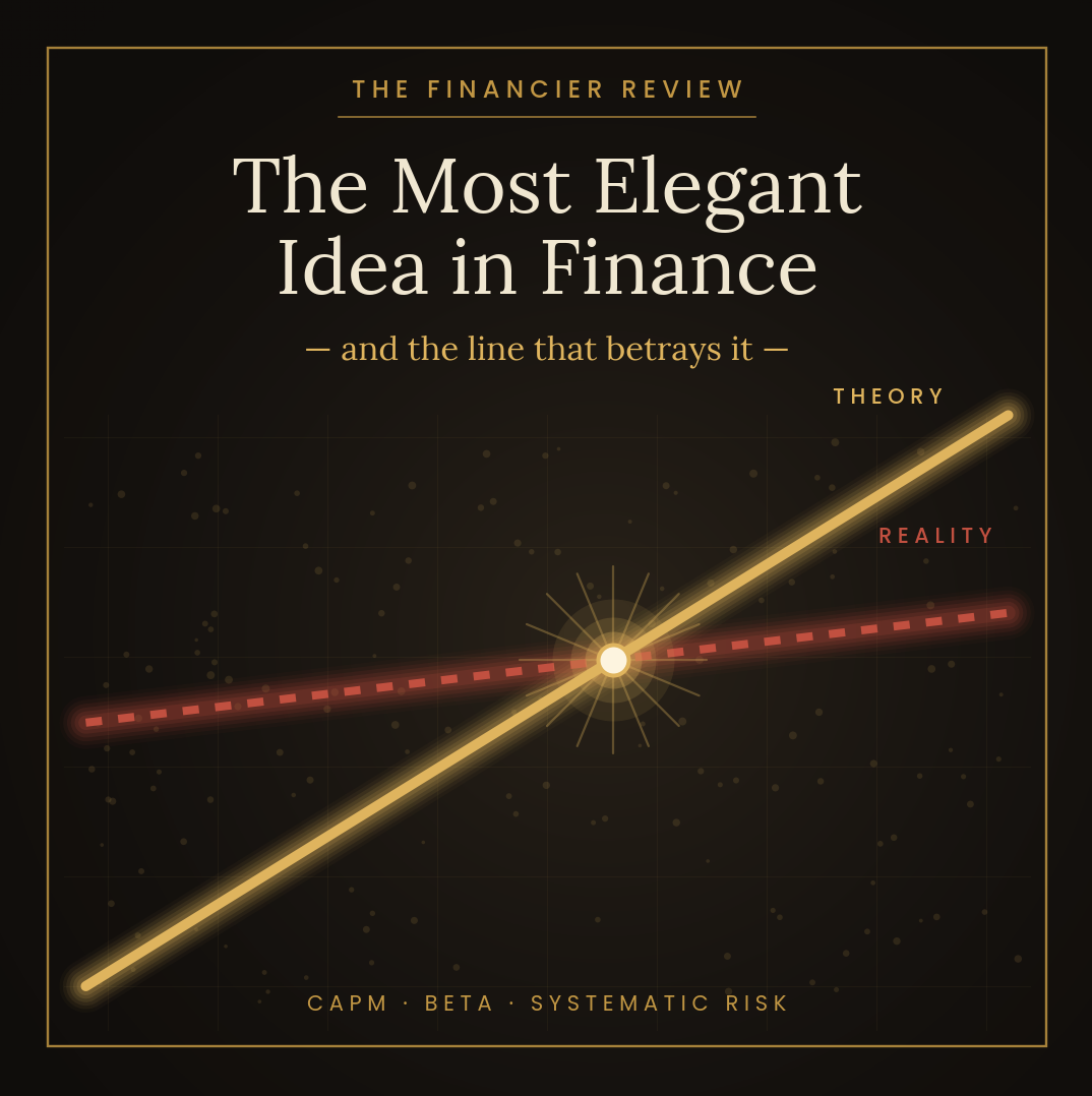
“CAPM is based on the first principle of finance: extra returns mean taking extra risks.”
A field guide to CAPM, beta, and the gap between theory and the tape.
Act I – The Elegance
There is a single equation, no longer than this sentence, that won a Nobel Prize, is taught in every finance programme on earth, and is fundamentally wrong. The infamous Capital Asset Pricing Model (CAPM), coined by the American economist William F. Sharpe (1964) gave a theoretical framework to calculate the rate of return on the asset based on its sensitivity to risk that is non-diversifiable. If we want to dive deeper into the concepts behind the theory for CAPM, we must distinguish beforehand between the two types of risk on an asset. The split is involving systematic and idiosyncratic (non-systematic) risk, where we concern ourselves with entire market (systematic) risk, specifically.
In an elegant manner the Capital Asset Pricing Model assumes that a rational investor would be able to almost eliminate non-systematic risk caused by single market events that would influence the price of an asset. Further, as well as having the ability to do so, out of rationality an investor would ideally diversify and eradicate idiosyncratic risk. An example of such could be considered holding a few stocks from public companies which would be subject to volatility from specific market events. If we investigate the stock of the famous Dutch corporation ASML Holding N.V. As of 2026 the company holds a very powerful near monopoly over the manufacturing of extreme ultraviolet (EUV) lithography machines. Such machines are currently the cornerstone to mass-production of the world’s most advanced semiconductor chips. The point to be made here is that even though this multinational giant holds quite practically a monopoly over the production of said machines they are susceptible to discrepancies in their supply manufacturing chain. Considering the intricacy involved in the production of such cutting-edge technology it is important to mention that constructing such a machine requires components from over 5,000 individual suppliers, which by themselves hold monopolies over their specific part of market share. Observing the trend here, we can make a plausible assumption that the market for assembly is rather predisposed to specific risk.
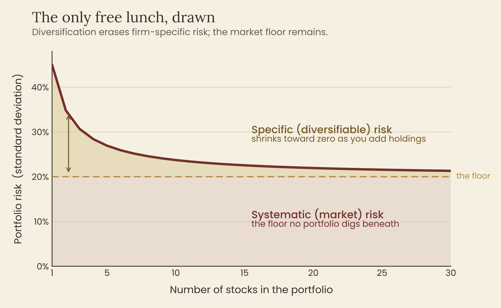
The company published quarterly results a day early, by accident, and the figures carried a brutal surprise: net bookings of €2.6 billion against a consensus near €5.6 billion — roughly half what analysts expected — alongside a cut to its 2025 guidance. The stock fell about 15.6% in a single session, its worst day since 1998, erasing nearly €50 billion in market value before lunch. Crucially, this was ASML's bad news, not the world’s. The broad European market barely moved that day; the damage was concentrated in one company's order book and one company's guidance. That gap — a stock in freefall while the index shrugs — is what specific risk looks like when it arrives. And it is precisely the risk a diversified investor never has to bear. Hold ASML inside a basket of two hundred names and that 15.6% blow lands as a rounding error. Therefore, since this type of risk is easily avoidable the market pays off very little to investors taking on this risk.
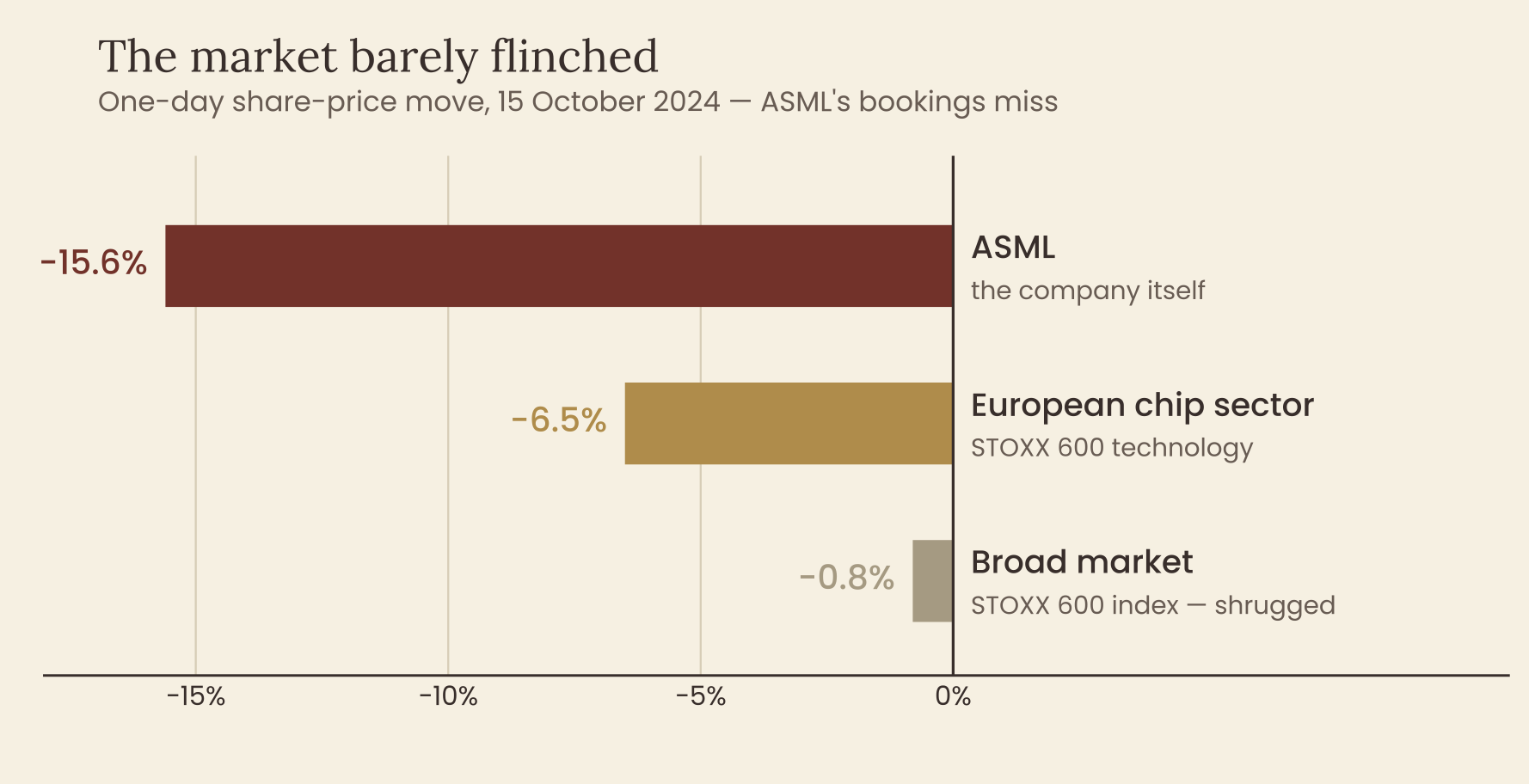
Having considered all this we can safely assume that a rational investor would hold multiple investments with some fractional shares, fully diversifying. We saw that singular market events that dropped the share price of the Dutch tech giant, had almost no influence on the broad market, let alone the global financial market. Well systematic risk is quite the opposite of what idiosyncratic risk is – it is the risk that belongs to everything at once. It is the type of force that would move the entire market as a whole. Under that notion, having more stocks, or generally more investments would make no difference to the potential losses that an investor would incur, in a crisis event.
While textbook cases of systematic risk frankly do not exist, some of them get very close to said definition, but we can work on the premise of which events are usually culprits for non-diversifiable risk. A simple adjustment of interest rates on behalf of a central bank could affect investing and re-price everything at once. Further, major economic and geopolitical crises like recessions and inflation shocks are also very typical backbones of systematic risk. Of course, we can spread risk further into wars, geopolitical ruptures and financial crisis, such as the 2008 Subprime Mortgage Crisis (The Global Financial Crisis).
To give dimension to systematic risk we can observe market behavior in March of 2020 – COVID. Since Covid-19 was declared as a global pandemic the market fell by about one third in just a month’s time and even more so, safe names and assets went down as well, with the whole market. With the introduction of such risk, despite attempts for elimination it is frankly impossible for diversify out of a total market “quake”. An even richer and more vivid example is 2008 – a breaking point where everything suddenly became correlated.
Now, it leaves us with a fundamental question to unravel here: if specific risk is purgeable through some form of diversification and as we discussed prior, systematic risk cannot. Logically the market would only reward the second type of risk – but to be precise we will need some form of measure on how much systematic risk a single stock has.
"Total risk = specific + systematic"
Thus, a stock’s risk comes in two flavours: some part that is unique to the company itself, or the single business market, and the part which it shares with the entire financial market. In our case, total risk is not a third category but just sum of the individual risk and the risk specific to the stock. But notice how what we stated are just classifications that tell us nothing about the individual risk carried by each stock, or how exponentially quickly the first type of risk disappears as we continue to diversify. Well, to turn this concept into something that we can utilize as measurement and subsequently price we need to go in the footsteps of Harry Markowitz in 1952.
Markowitz’s Idea Put in Numbers
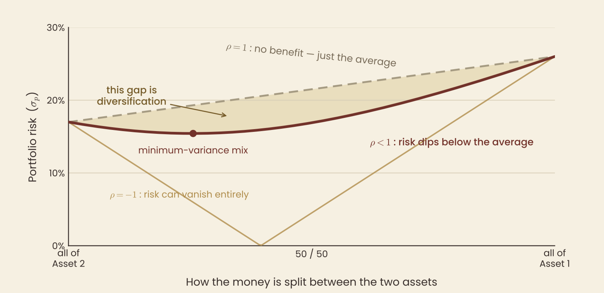
Hence, what did Markowitz do? He stopped thinking about stocks as a singular event and looked at them as how they move together. The moment you materialize this though in numbers, a surprising concept appears. Risk does not add up the way funds do. If we consider two stocks in the same portfolio their cumulative average risk is not the average of the two individual risks – it is usually less. So, the theory suggests this two-asset version as a sort of landmark for the shape of the idea.
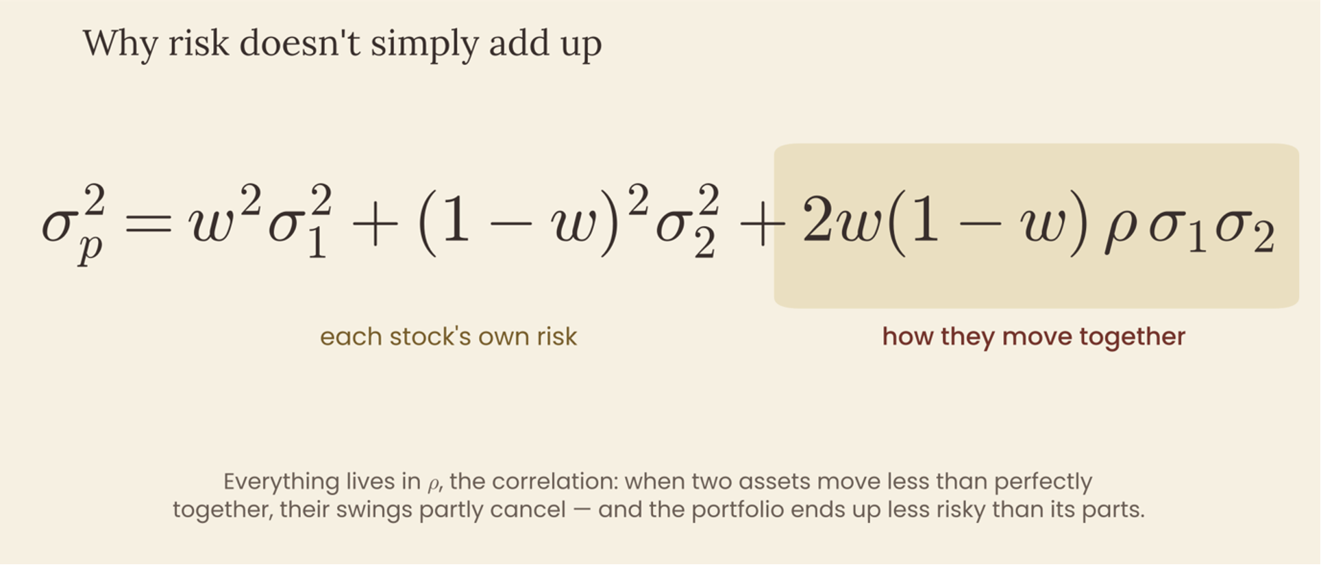
In general, everything that is intriguing to us is situated in the last term of the equation – ρ. Mathematically – if they move in perfect synchronization (ρ=1) there is no benefit and the actual cumulative risk of the two assets is just the average. But the story becomes completely different when they move in a less than perfect matter (ρ<1) – their returns are imperfectly correlated, so a portion of each one’s variance is offset by the other’s (the ups and downs cancel) leading to a drop below the average of its parts. Put simply, the cancellation of these two variances is in practice diversification.
Scaling the Two Asset Model Up
Now imagine the following: if we can model the risk movement of two stocks and cancel out specific risk, through analyzing their correlation, can we do the same for many more stocks. Without a question the model begins to show its strengths with the introduction of many stocks at the same time. To achieve mathematical reliability, we need to scale the model up using a factor. We take a portfolio of n stocks and split evenly between each stock. From here the variance (how far the numbers spread from the mean) splits in two formula pieces.
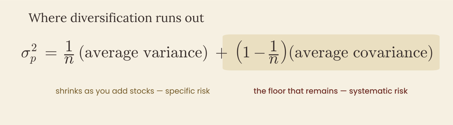
At a first glance this seems like a straightforward concept with nothing intriguing but notice something strange happening with the terms. Watch what happens as the term n grows, or in other words we add more stocks. Do you recognise this graph from a few paragraphs above? The more stocks we add (diversify), with an exponential decay the specific risk plateaus to near 0. The first term of the equation (1/n)· (average variance) carries what we call every stock’s risk. It’s then divided by n so it converges it to zero.
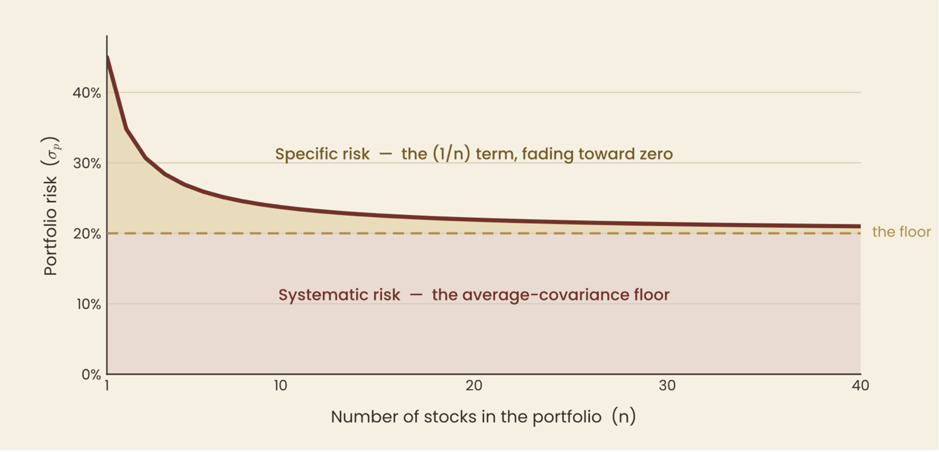
Exploring the second term of the equation (1 − 1/n)· (average covariance) we can model how the stocks, bundled together move. As n grows the term (1 − 1/n) approaches 1. The term itself does not disappear, but it settles onto the average covariance of the joint movement and stays there. With that said we can enforce the idea that the limit for a portfolio that is well spread out and large in individual stock volume is the average covariance
Limit as n approaches infinity -> σ²ₚ → average covariance.
With all the aforementioned mathematics we can make a very simple deduction and extract the essence of the idea behind the model. As you diversify a portfolio, each stock’s individual risk cancels out entirely. With the division by n the individual risk disappears. What is left at the bottom of the graph – a rectangular shape that refuses to go away, with no effect to the number of individual stocks an investor holds are the stocks moving together. In other words, these seemingly separate ideas crumble into two main points.
The term that decays to zero as n grows is what we defined as specific risk – a type of risk that can be mitigated through diversification. The floor, which we cannot get rid of is so called systematic risk. And back to our original equation:
"Total risk = specific + systematic"
The Collapse of The Model to a Single Line.
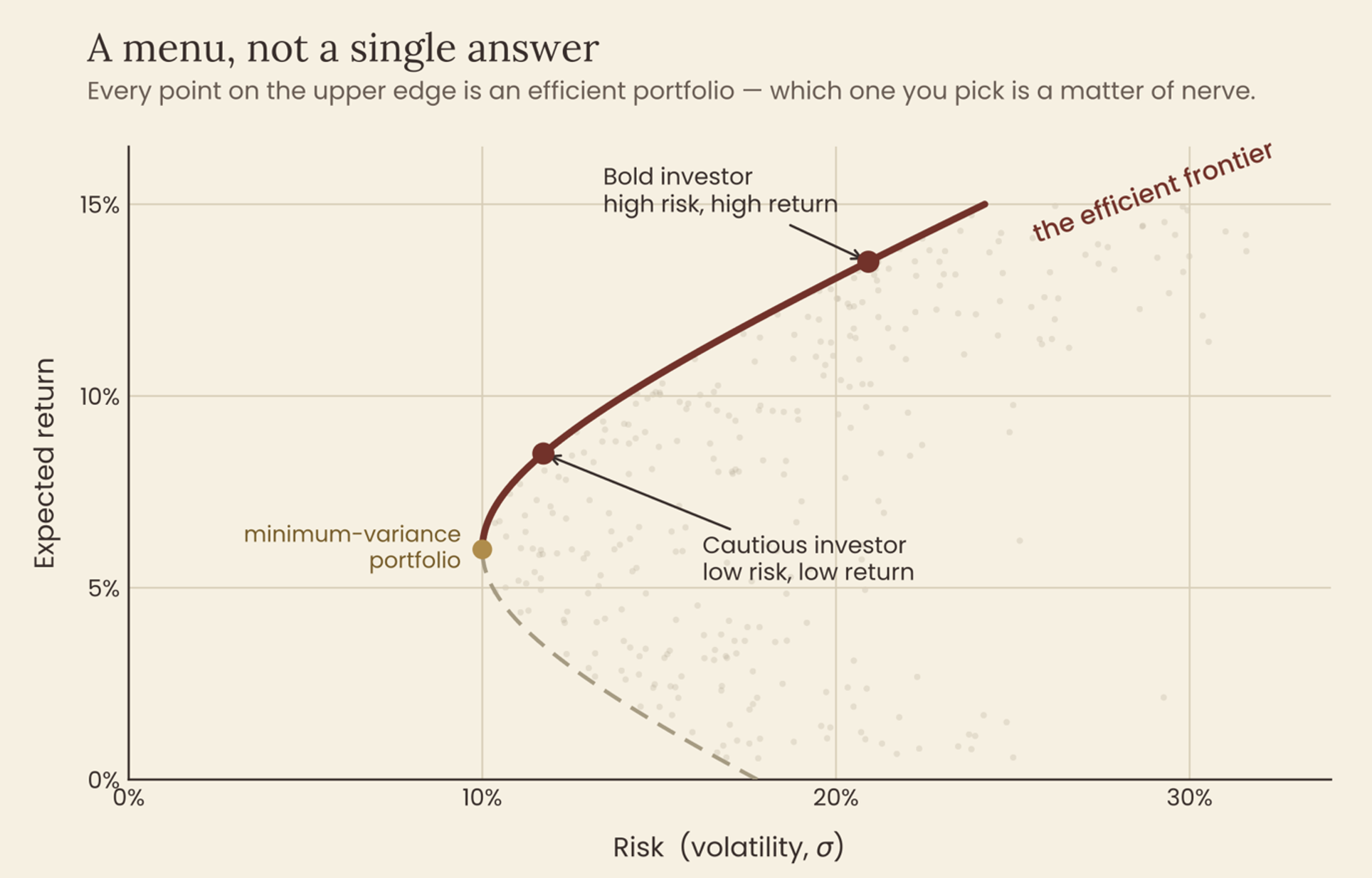
So far from Markowitz notion we have a curve. The curve, also known as the efficient frontier, gives an investor a selection menu of the best-achievable portfolios. Picking one type of bundle depends on your risk appetite. A cautious investor will be situated on the bottom left of the graph and a more risk oriented, bold investor would be on the top right. Depending on each individual investor and their willingness to take risk, they opt out for different portfolios. Seem reasonable enough, right? Well not quite.
Then another American economist by the name of James Tobin, in 1958, added the one ingredient which gave a whole new perspective to the original model. That ingredient is factor called a risk-free asset. Such class of assets is considered more on the theoretical side but in principle they are investments that guarantee completely predictable returns with no credit or default risk. Government debt is usually considered to be such an asset. A simple explanation follows that the chance of a government to not repay you back is almost none. As follows, the moment you can lend or borrow at a safe rate that is consistent and predictable, the elegant frontier curve is replaced by a single straight line. The line is drawn from the risk-free rate (set at 0) to a single tangent point with the frontier. By definition this graze point is a specific portfolio, developed by risky assets.
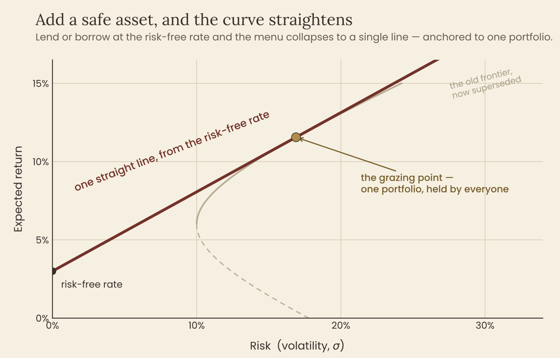
The less intuitive part to this idea is the implication that a single tangent point means that everyone now holds the same portfolio. Well, this phenomenon is called Tobin’s Separation Theorem. In other words, you might think that a more nervous investor’s portfolio would be different from a risk taker’s one, but you would be wrong. Theoretically, they own the same risky portfolio, and the only difference is the split between cash and the risky portfolio. A more cautious investor would contain a large portion of their capital in safe assets and put the rest in the risky portfolio. Accordingly, the risky investor borrows at the risk-free rate and allocates more than their own money in the exact same risky portfolio. Risk appetite does not decide what you own, but more of how much exactly you should own.
Identifying the Tangent Portfolio
We have given way to naming the exact notions behind choosing this portfolio, but we still have no idea what that exact portfolio would look like. William Sharpe gave an answer to this question in 1964, and the underline logic is very intuitive and clean. If every investor on earth holds the same basket of risky assets, then that basket has to contain everything — because every share must be owned by somebody. The one portfolio everyone holds can only be the market itself : every asset, weighted by its size.
Subsequently, since the entire market is the universal portfolio itself the fundamental model divides into two very direct statements. For our efficient portfolios on the frontier, Tobin’s line would be named the Capital Market Line.
This relationship is modeled by the following equation:
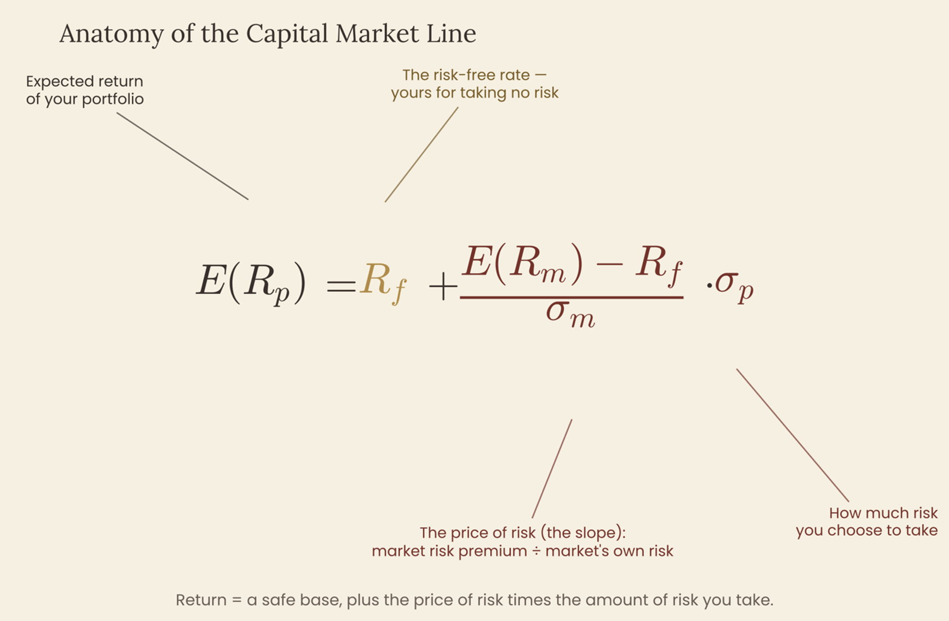
Thus, the slope of this equation is the entire market’s reward-to-risk ratio. What is the price of risk for the entire economy but materialized as a single number. But as mentioned, here we measure the risk for the entire economy. To model accurately, we would also need the risk for an individual asset. We measure the risk for an individual asset by beta ( β ). In other words, the sensitivity of the asset to the market’s movement.
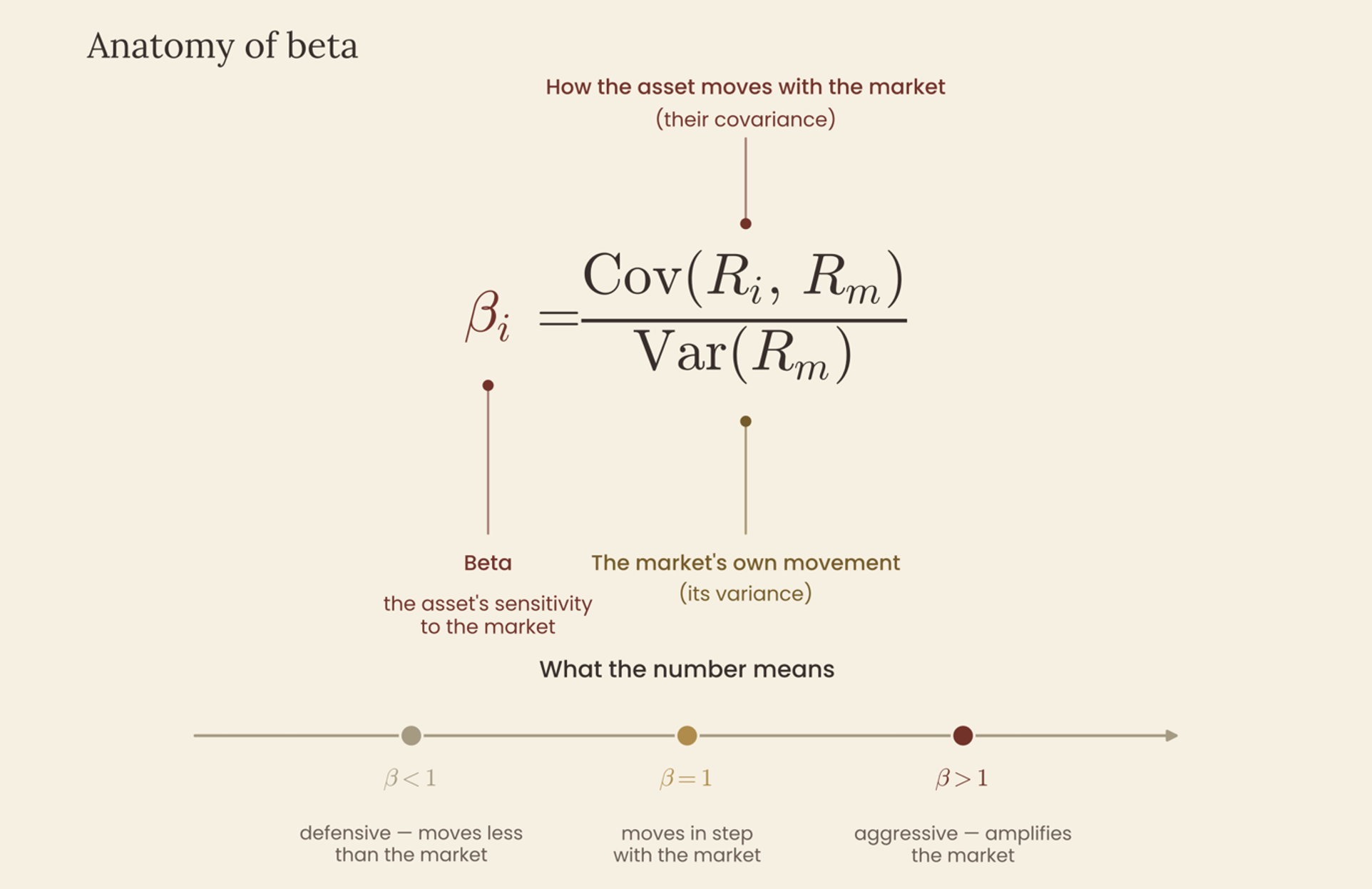
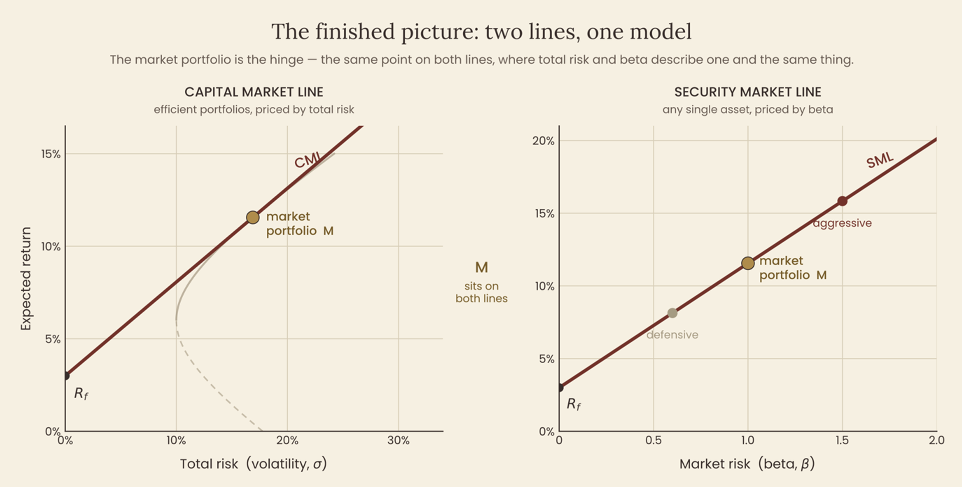
When we feed the equation for the sensitivity of an individual asset into the equation that models the risk for the entire market economy, we reach the Security Market Line (SML). An important point to raise attention here would be why do we use beta, and not volatility? Prior, we measured the risk of a portfolio by its total volatility given a term σ, but here for a single asset we use a different measure – beta. Looking back at the mathematics behind diversification – an investor holding the market has already diversified fully each asset’s individual stock volatility. It was the term (1/n) that fades away to nothing. So considering a stock’s own fluctuations is irrelevant, since they are already cancelled. Thus said, the only risk that could be reasonably priced is the portion of the stock that contributes to the market movement – with that contribution being beta.
In other words, the Capital Asset Pricing Model is not a fundamentally new principle, but one which is the diversification result, followed to its logical conclusion. An individual asset has its own volatility, which is diversifiable and underpriced since it is so easily avoidable. With systematic risk, it is the sensitivity of the asset, with the risk being unmitigable and objectively priced.
Birdseye View of The Model
Now, here is how we would position the development of this theory. While Markowitz needed the entire web of relationships between assets with every variance, covariance equation to thousands of numbers to model risk, CAPM mandates only one parameter per asset – Beta. The entire matter of risk is reduced to a single straight line for the market and a letter that mirrors everything.
At this point this is the moment of the CAPM theory where it is most elegant. It is the foundational complete answer to a problem which seems unsolvable and explainable in a breathtakingly compact way. The most elegant idea in finance.
But unfortunately for elegance, data shows up…
Act II – The Betrayal.
The Line that is Simply too Flat
Remember the line you just fell for. Expected return rising in a straight shot from the risk-free rate, climbing at exactly the market's premium — one clean prediction, neck stuck out, daring the world to check it. So, let's check it. If we were to classify every stock with their respective beta, sort and plot we would find that the line is real. A higher beta (an amplifying stock) correlates to a higher payout. The issue with this is that at a first glance nothing seems wrong, but the truth is that the line is just too flat. Next, we want to imagine that somebody would flip the ends of the line in a way that low-beta stocks land above the model point and high beta below. This translates to something very concerning – safe and boring stocks fly under the radar and beat the model, while exciting, risky stocks underperform. But how is that even possible? Is it truly the case in practice? The line isn’t exactly off in the corners. The issue lies in the foundational function to price beta itself.
Since seeing and reasoning with all of the elegant math surrounding the model, stating such a powerful claim about a seemingly “super reasonable” principle seems absurd, but in practice it isn’t. People caught the discrepancies almost the moment data started existing and became analyzable. We are referring to a period of within a decade of the model’s birth. This fantastic principle was technically broken and still is yet it kept running the markets and even to this day is a widely used model.
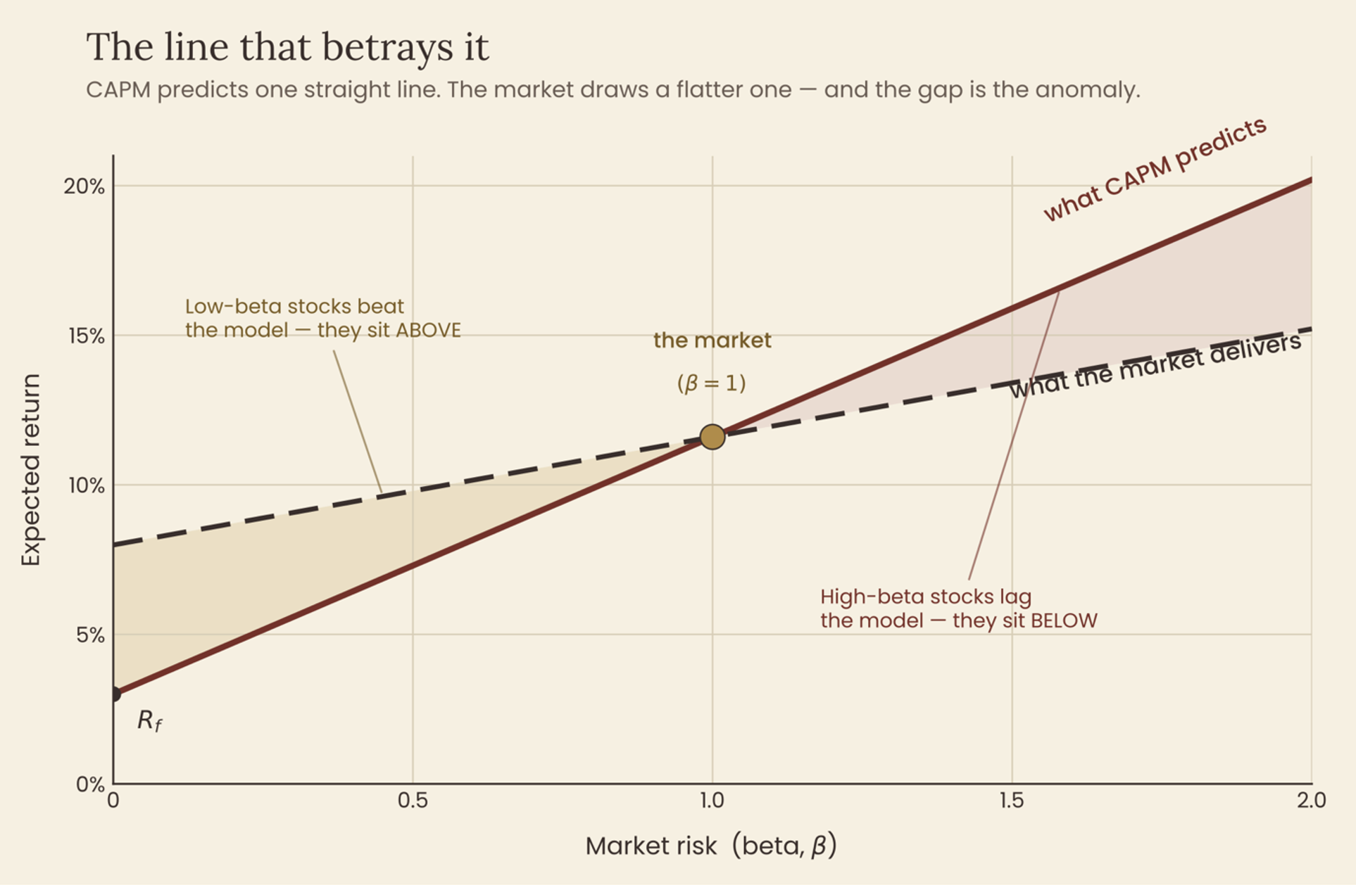
Since the data points in the direction of the graph above and in principle the model is incorrect with pricing beta, can we take any other reasonable and most importantly profitable conclusions? Frazzini and Pedersen wrote in 2014 that we buy the underpriced low-beta names, lever them up, short the overpriced high-beta ones, and pocket the gap the model left on the table. Further, they also tell you why the gap is there and answer to this question is something we already met with. The majority of investors cannot or would not borrow, a fund’s mandate does not allow it, and the margins frighten them therefore the option is simply not feasible. Following, when they do decide they want a higher return they cannot leverage something safe, so they resort to high beta stocks instead. By the law of supply and demand – an increased demand for an asset raises the price and by relation, safe assets are left with lower prices. In practice that is the flattened line.
Why don’t we go back to the fundamentals of CAPM? The line that we draw in the first place, the one which shows that everybody could borrow freely at a risk-free rate – Tobin’s move. If we take this assumption away, the newly formed line bends exactly the way the data suggests. So, the betrayal of this model was never something external, but it was the “devil” hiding in the preliminary assumptions.
If you still doubt this financial model, we can take a look at what is sold on the market nowadays. There are entire funds with “low volatility”, “mid-level volatility” and whatever other kind of label they manage to identify with – all built and marketed on this single flaw. A broken theory is supposed to embarrass quietly. This one has a marketing budget. When an industry packages your model's failure and sells it back to investors, the model hasn't just been proven wrong. It's been monetized against.
The Roll Critique: A fundamental limitation.
Some 13 years following the official publication of CAPM, an economist by the name of Richard Roll discovered a fundamental flaw in the foundation of the model. While the flat line was an empirical problem, this next issue is more of a philosophical one. The core problem with which the work of professor Roll concerns itself is that CAPM is built on one object. That object is the market portfolio which includes every risky asset on earth. The truth is that it is impossible to observe a true market portfolio. One would include not only all stocks, but also all bonds, private businesses and even human capital. Truthfully, it is impossible to measure the true market portfolio therefore nobody has managed to test CAPM on the perfect definition of a real market portfolio.

Prof. Richard Roll, Ph.D. in economics, finance, and statistics.
The silent blade in this crack is the fact that most tests of CAPM include something known as a stand-in. In the literal sense it is a substitute for the perfect notion. Therefore, CAPM usually gets tested on a stand-in such as the S&P500 or the Nasdaq. So Richard Roll’s point is very logical and conclusive: in case a test fails to support CAPM, it is impossible to tell whether the model was inaccurate, or the stand-in is not representative of the market, because it is based on sampling the true market portfolio, not its actual entirety.
What is unsettling as an implication to this very logical observation made by the American economist Richard Roll is that CAPM isn’t just possibly wrong, but also practically untestable. Fundamentally, a deeper failure than just the model being false – an inaccurate theory can at least be rejected cleanly. With the Capital Asset Pricing Model, it isn’t just potentially false, but also this one can’t even be put fully to trial.
Does Beta even work? – Fama-French Crack.
If Richard Roll inquired whether CAPM can truly be tested, the scholars Eugene Fama and Kenneth French asked a more specialized question: does beta really work? Is it really a reliable measure of a stock’s sensitivity to the market, and are there any inaccuracies?
Well after sorting the stock market meticulously, the two economists discovered that beta has an astonishing inaccuracy to explain why some type of stocks on average yield a higher return, compared to others. They found that two other factors contributed much more to the accuracy of return that beta: company size and value. In essence, smaller companies tend to outperform larger ones and with value, a low price relative to fundamentals tends to beat more expensive ones.
In practice this issue is mitigated through the addition of those two variables as separate factors, turning CAPM’s single number principle into a three-factor model. Of course, with the increased reliability and the introduction of multiple variables the model becomes much harder to trace and less easy to use. The three-factor model introduced in 1993 utilized a size factor by the name of SMB (Small minus Big), or in other words the historical tendency for small enterprises to provide higher returns than larger ones. HML (High minus Low), or the second additional parameter was concerning itself with the tendency of cheap stocks to outperform expensive ones – the value parameter. Therefore, as a result of all this the expected return on a stock is now dependent not only on its sensitivity to the market (beta), but also to the size and value effect.
About two decades later the team introduced an even newer and revised model. In 2015 Eugene Fama and Kenneth French they revealed an extended model which now added 2 parameters to the already 3 available, giving a total of 5. The mentioned factors are a firm’s profitability and investment practices. Companies which have more profit naturally provide better returns than lower profit ones. Subsequently, enterprises with more conservative investment strategies tend to outperform very aggressive firms. At some point following the introduction of the 5-parameter model, researchers suggested including even more factors and the whole idea became somewhat of a joke in the financial research world. Nicknamed the “factor zoo” where more and more factors are included.
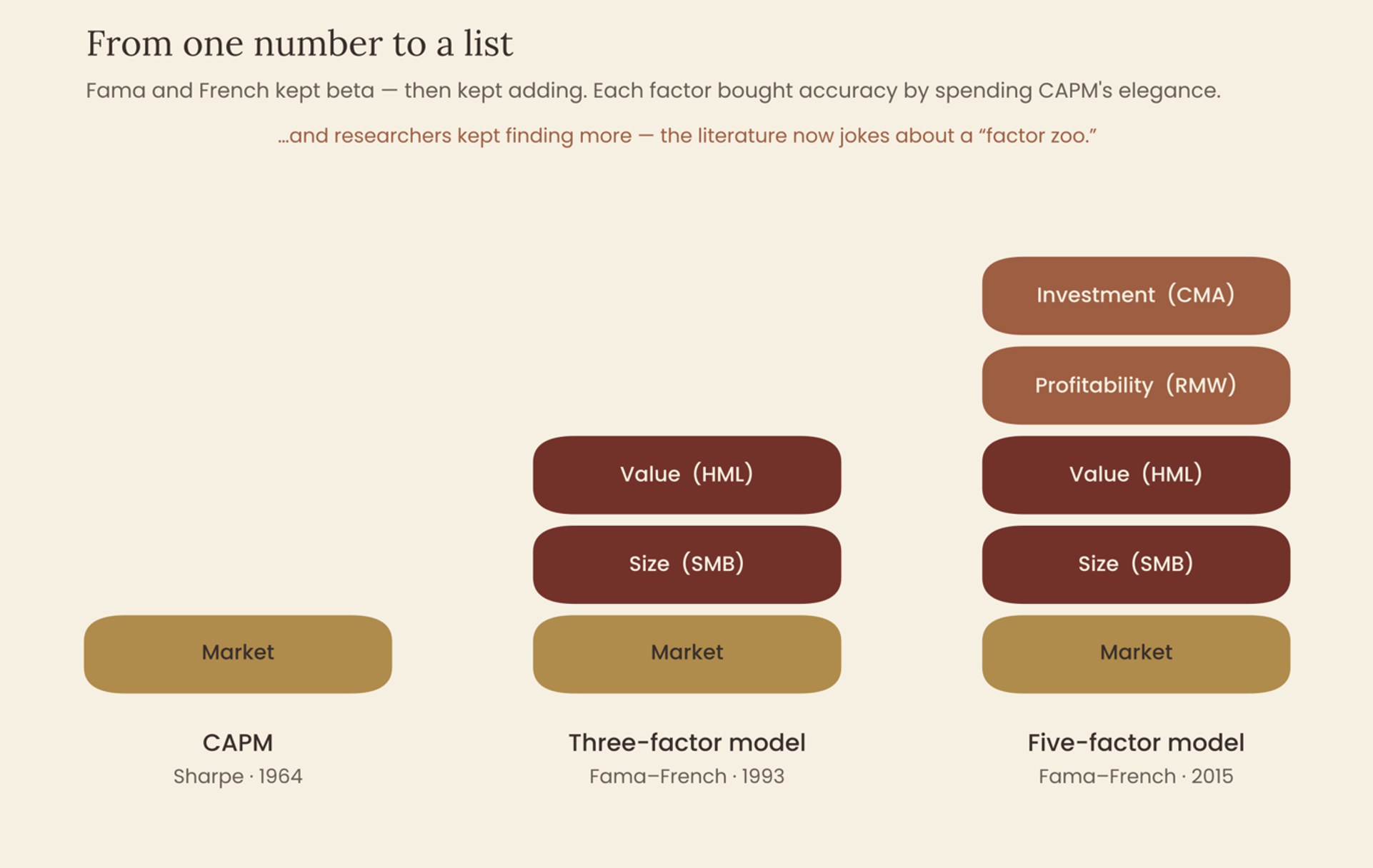
But with all that, there have been many instances of criticism towards CAPM and its simplicity, but the truth is that the model provided a foundational framework. While it might not be the most efficient or accurate, the whole appeal of it is that it captured an important piece of information about a stock in just a single number. We notice that the model did not get “fixed” in the traditional sense, but it expanded. Each additional factor to the model allows for more accuracy and includes omitted layers to the equation. Every new additional patch sacrificed on the elegance of the Capital Asset Pricing Model but brought accuracy. The elegance which made the model worthy in the first place.
Act III – The Reckoning
The Last Man Standing.
So, we explored how CAPM was developed, it’s building blocks and we also saw how fundamentally flawed the model is. Following a logical conclusion to our exploration – why is CAPM still the first concept taught in every finance class? It is still the number on every cost-of-capital calculation. The model was falsified and deemed untestable within a decade, outperformed in accuracy by more complex, messier models – so what is in it for us with the Capital Asset Pricing Model?
Well, if we look at this model as a kind of language, with its own vocabulary, rather than a bullet-proof law it starts to make sense. It gave us a pathway to reason and understand that risk and return are linked by a line. Some type of risk is rewarded, and some isn’t. We also understood that an asset’s risk is its relationship with everything. The value is not in the predictions of the model itself, but in the way it taught us to observe and talk about risk. A wrong theory that reorganizes how a field thinks is more durable than a right one that doesn't. CAPM is wrong the way Newton is incorrect – superseded in precision, indispensable as a foundation.
The Coda: From Theory to Money.
Arguably, the most difficult implication to be derived here is that with a flawed model that is too basic to be practically useful, can the average investor really benefit? The answer to this question is not yes in the traditional sense. It isn’t a textbook answer, but there are some very useful lessons to be learned here.
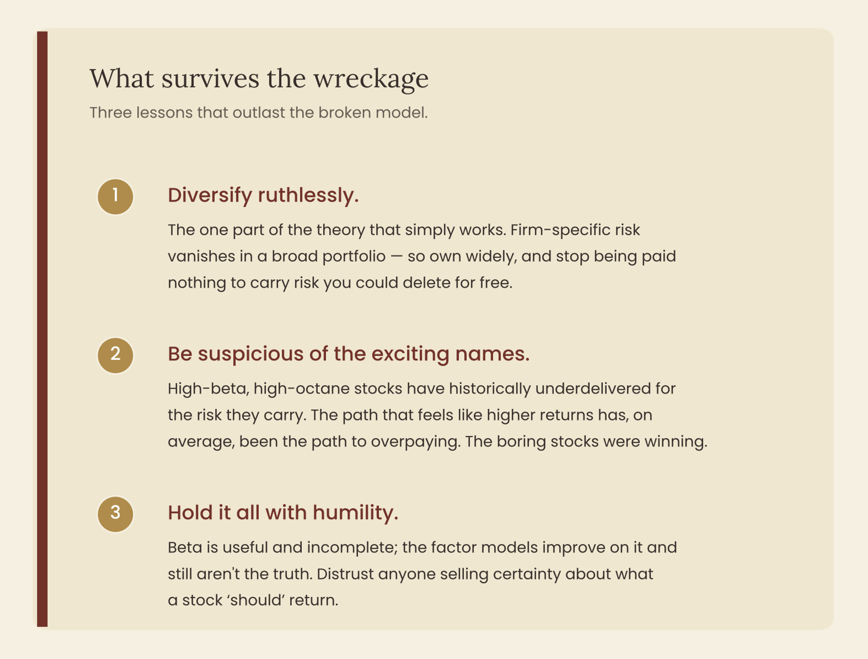
To finalize this story about how simplicity allowed us to create something that is fundamentally flawed, but the elegance of the notion gave a path to something greater. While CAPM is technically incorrect at pricing risk, and it did get its central line wrong we do use it anyway. Not despite that, but because being usefully, beautifully wrong is in many instances the most we could hope for in a theoretical model. The line betrayed it. The idea outlived the line.
References
Black, F., Jensen, M. C., & Scholes, M. (1972). The Capital Asset Pricing Model: Some Empirical Tests. In M. C. Jensen (Ed.), Studies in the Theory of Capital Markets (pp. 79–121). Praeger.
Fama, E. F., & French, K. R. (1992). The Cross-Section of Expected Stock Returns. The Journal of Finance, 47(2), 427–465.
Fama, E. F., & French, K. R. (1993). Common Risk Factors in the Returns on Stocks and Bonds. Journal of Financial Economics, 33(1), 3–56.
Fama, E. F., & French, K. R. (2015). A Five-Factor Asset Pricing Model. Journal of Financial Economics, 116(1), 1–22.
Fama, E. F., & MacBeth, J. D. (1973). Risk, Return, and Equilibrium: Empirical Tests. Journal of Political Economy, 81(3), 607–636.
Frazzini, A., & Pedersen, L. H. (2014). Betting Against Beta. Journal of Financial Economics, 111(1), 1–25.
Lintner, J. (1965). The Valuation of Risk Assets and the Selection of Risky Investments in Stock Portfolios and Capital Budgets. The Review of Economics and Statistics, 47(1), 13–37.
Markowitz, H. (1952). Portfolio Selection. The Journal of Finance, 7(1), 77–91.
Mossin, J. (1966). Equilibrium in a Capital Asset Market. Econometrica, 34(4), 768–783.
Roll, R. (1977). A Critique of the Asset Pricing Theory's Tests Part I: On Past and Potential Testability of the Theory. Journal of Financial Economics, 4(2), 129–176.
Sharpe, W. F. (1964). Capital Asset Prices: A Theory of Market Equilibrium under Conditions of Risk. The Journal of Finance, 19(3), 425–442.
Tobin, J. (1958). Liquidity Preference as Behavior Towards Risk. The Review of Economic Studies, 25(2), 65–86.
All data used in this article is derived from publicly available institutional reports and industry analyses.
This article is for informational purposes only and does not constitute investment advice.
Mihail Gaydarov
Founder & Chief Financial Analyst.
The Financier Review
© 2026 The Financier Review. All rights reserved.
